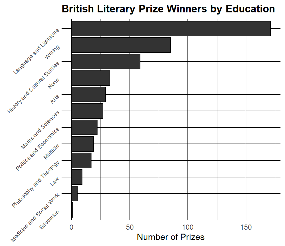
This particular project utilized a data set consisting of personal information from winners of various noteable literature prizes over time. As someone who almost chose English as a college major, I thought it would be interesting to see what the “best” education is for an author. Obviously these results are skewed, as those who already enjoy writing are more likely to take subjects related to it in post-secondary education.
I enjoyed the use of the distinct() function here as it was not something I had used prior.
prizes <- prizes |> distinct(person_id, .keep_all = TRUE)

All of the code for this project is shown below:
library(tidyverse)

#import data
prizes <- readr::read_csv('https://raw.githubusercontent.com/rfordatascience/tidytuesday/main/data/2025/2025-10-28/prizes.csv')

#remove any duplicates (this could be skipped, I wanted to try distinct())
prizes <- prizes |> distinct(person_id, .keep_all = TRUE)

#create new data structure with the number of prizes for each education type
table <- prizes |> count(degree_field_category)

#remove entries lacking information
table2 <- subset(table, degree_field_category != "unknown" )

#fix formatting of "none"
table2 <- table2 |> mutate(degree_field_category = if_else(degree_field_category == "none", "None", degree_field_category))

#graph
ggplot(data = table2, aes(x = n, y = reorder(degree_field_category, n))) +
geom_bar(stat = "identity", color = "black", fill = "grey20") +
labs(x = "Number of Prizes", y = NULL) +
theme_minimal() +
ggtitle("British Literary Prize Winners by Education") +
theme(
  axis.text.y = element_text(angle = 45, hjust = 1, size = 7),
  plot.background = element_rect(fill = "white"),
  panel.grid = element_line(color = "black"),
  plot.title = element_text(face = "bold", hjust = 0 ))